A first example

Let us first illustrate the most commonly useful features of Manopt using a standard optimization problem on a sphere.

The math

Let \(A \in \mathbb{R}^{n\times n}\) be a symmetric matrix. The eigenvectors of \(A\) associated to its largest eigenvalue are known to be the optimizers for the following optimization problem:

\[\max\limits_{x\in\mathbb{R}^n, x \neq 0} \frac{x^\top A x}{x^\top x}.\]

The cost function is insensitive to the norm of \(x\), hence we might as well fix it to \(x^\top x = \|x\|^2 = 1\). Also, we would like to have a minimization problem rather than a maximization problem (we’ll see why in a moment). Accordingly, we flip the sign of the cost function. In the end, we want to solve:

\[\min\limits_{x\in\mathbb{R}^n, \|x\| = 1} -x^\top A x.\]

The cost function and its gradient in \(\mathbb{R}^n\) are:

\[ \begin{align*} f(x) = -x^\top A x, && \nabla f(x) = -2Ax. \end{align*} \]

(See the matrix calculus website for help with figuring out gradients. You can also learn the math to do these computations in Section 4.7 of this book.)

The constraint on the vector \(x\) tells us that \(x\) is a point on the sphere (one of the nicest manifolds):

\[\mathbb{S}^{n-1} = \{x \in \mathbb{R}^n : x^\top x = 1\}.\]

This is all the information we need to apply Manopt to our problem. For additional theory, see the cost function page and the learning page.

The code

Solving this optimization problem using Manopt requires a few lines of Matlab code. Here they are, and explanations follow.

% Generate random problem data.
n = 1000;
A = randn(n);
A = .5*(A+A');

% Create the problem structure.
manifold = spherefactory(n);
problem.M = manifold;

% Define the problem cost function and its Euclidean gradient.
problem.cost  = @(x) -x'*(A*x);
problem.egrad = @(x) -2*A*x;      % notice the 'e' in 'egrad' for Euclidean

% Numerically check gradient consistency (just once, optional).
checkgradient(problem); pause;

% Solve.
[x, xcost, info, options] = trustregions(problem);

% Display some statistics.
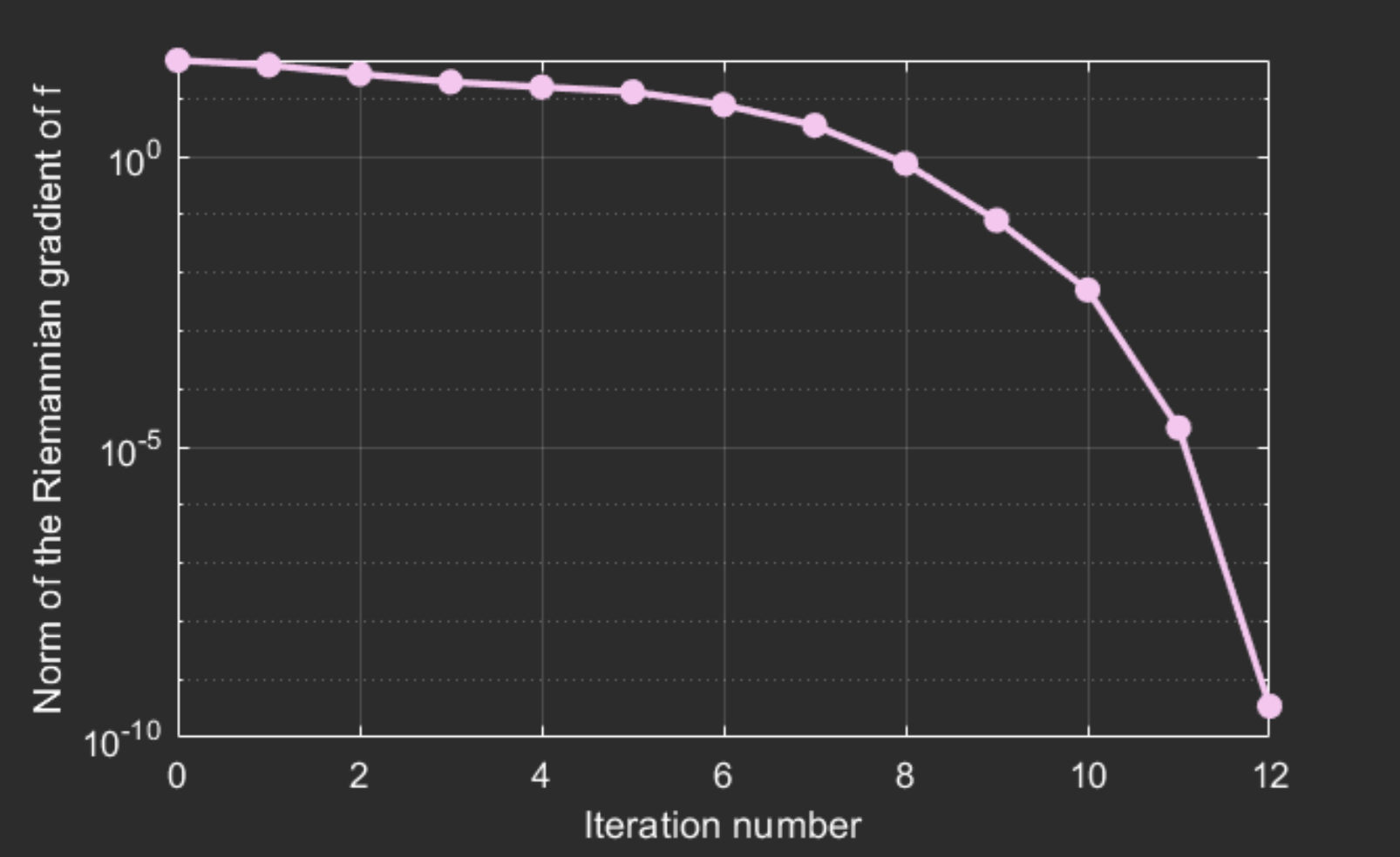
figure;
semilogy([info.iter], [info.gradnorm], '.-');
xlabel('Iteration number');
ylabel('Norm of the Riemannian gradient of f');

Let us look at the code bit by bit. First, we generate some data for our problem. Then, we execute these two lines:

manifold = spherefactory(n);
problem.M = manifold;

The call to spherefactory returns a structure describing the manifold \(\mathbb{S}^{n-1}\), i.e., the sphere. This manifold corresponds to the constraint appearing in our optimization problem. For other constraints, take a look at the various supported manifolds.

The second instruction creates a structure named problem and sets the field problem.M to contain the manifold structure.

The problem structure is further populated with everything a solver might need to know about the problem in order to solve it, such as the cost function and its gradient:

problem.cost  = @(x) -x'*(A*x);
problem.egrad = @(x) -2*A*x;

The cost function and its derivatives are specified as function handles. Notice how the gradient was specified as the Euclidean gradient of \(f\), i.e., \(\nabla f(x) = -2Ax\) in the function egrad (mind the e). The conversion to the Riemannian gradient happens automatically behind the scene. This is especially useful with more complicated manifolds.

We could also define the cost and its derivatives in several other ways, e.g., to avoid the redundant computation of the product A*x: see the cost description page. In particular, with Manopt 7.0 and Matlab R2021a or later, if you have the Deep Learning Toolbox, then you can also use automatic differentiation (AD) instead of defining the gradient (and even the Hessian) yourself:

% problem.egrad = @(x) -2*A*x; -- we can replace that line with:
problem = manoptAD(problem); % automatic differentiation

See the cost description page for more information. Keep in mind that, while AD is convenient and reasonably efficient, it is usually slower than (good) hand-written code.

The next instruction is not needed to solve the problem but often helps at the prototyping stage:

checkgradient(problem);

The checkgradient tool verifies numerically that the cost function and its gradient agree up to the appropriate order. See the tools page for further details and more helpful tools offered by Manopt. This tool generates the following figure:

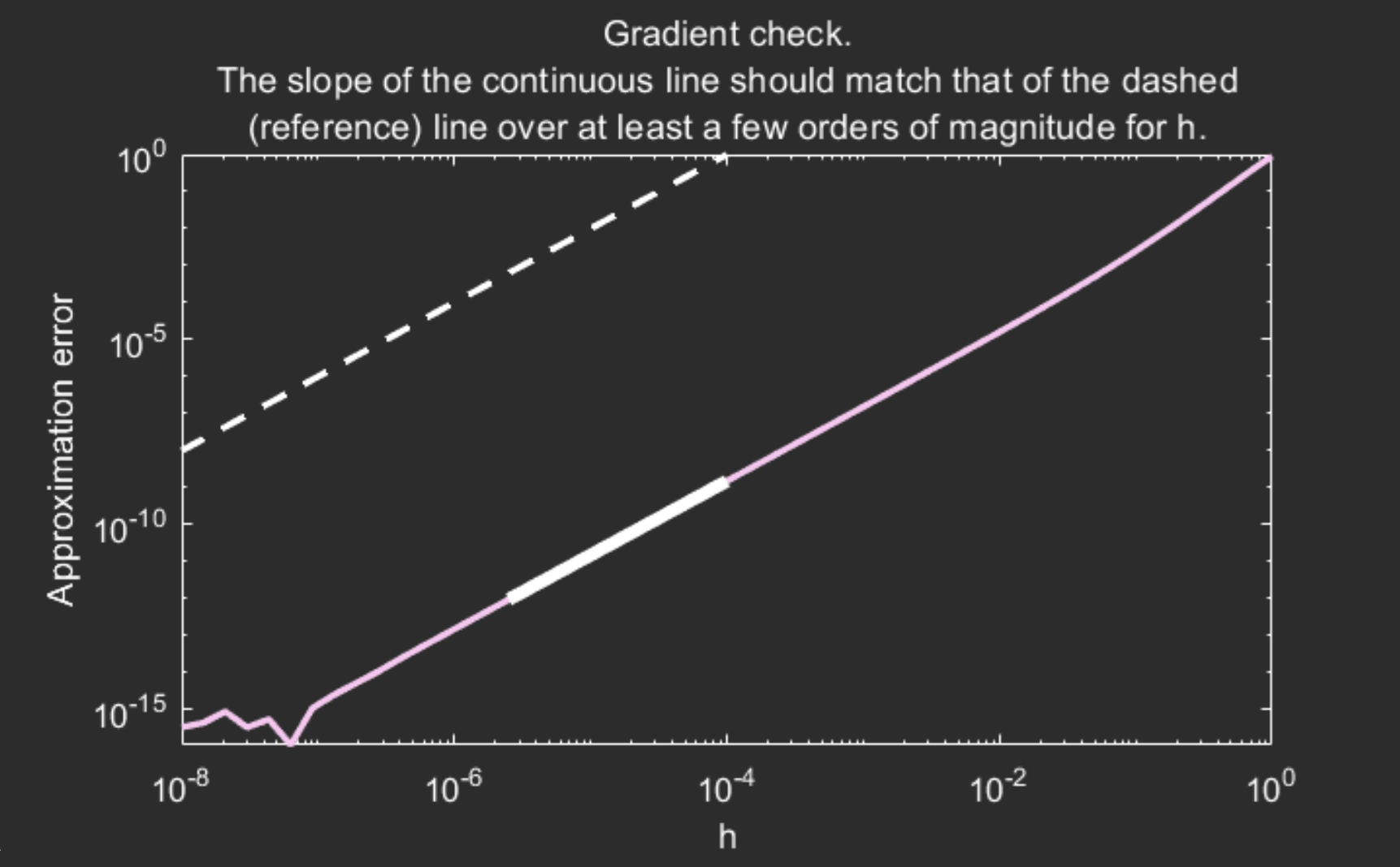
The `checkgradient` tool outputs a figure and text in the command line. In the figure here, we see that part of the continuous curve has a slope that matches that of the dashed line: that’s what we like to see. If not, then it is likely that the gradient is incorrectly implemented. Try it: change `problem.egrad` to `@(x) A*x` for example and see what happens.

The blue curve seems to have the same slope as the dashed line over a decent segment (highlighted in orange): that’s what we want to see. Also check the text output in the command prompt.

We now run one of the solvers on our problem:

[x, xcost, info, options] = trustregions(problem);

This instruction calls trustregions, without initial guess and without options structure. As a result, the solver generates a random initial guess automatically and resorts to the default values for all options. As a general feature in Manopt, all options are, well, optional.

Manopt always minimizes

All solvers in Manopt aim to minimize the cost function in the problem structure. If you want to maximize a function, do as we did earlier on this page: flip the sign of \(f\) (and likewise for its derivatives).

The returned values are:

x: usually an approximate local minimizer of the cost function,
xcost: the value of \(f\) at x,
info: a struct-array containing information about the successive iterations performed by the solver, and
options: a structure containing the options used and their values: peek inside to find out what you can parameterize.

For more details and more solvers, see the solvers page.

This call issues a warning:

Warning: No Hessian provided. Using FD approximation.

That is because the trust-regions algorithm normally requires the Hessian of the cost function to be provided in the problem structure. When the Hessian is not provided, Manopt approximates it using finite differences on the gradient and it warns you about it. This is mostly fine. You may disable this warning by calling warning('off', 'manopt:getHessian:approx');.

Finally, we access the contents of the struct-array info to display a convergence plot:

semilogy([info.iter], [info.gradnorm], '.-');  
xlabel('Iteration number');  
ylabel('Norm of the gradient of f');

This generates the following figure. For more information on what data is stored in info, look inside and see the solvers page.

The Riemannian gradient norm is converging to zero fast: that’s what we like to see.

info is a struct-array

Notice that we write [info.xyz] with brackets, and not simply info.xyz. This is because info is a struct-array. Read this MathWorks blog post for further information.

You may omit the gradient, but…

In the example above, we specified the gradient but not the Hessian. As a result, Manopt automatically uses finite differences (FD) to approximate the Hessian if needed. This is fine.

If we also do not specify the gradient, then Manopt approximates that with FD as well. The solver will run, but this is slow. The approximation is good enough that it is convenient to have as a feature for prototyping on low-dimensional manifolds, but it should not be used for anything serious. If you do, you may want to set options.tolgradnorm to a larger value (say, 1e-4) and pass the options structure to the solver.